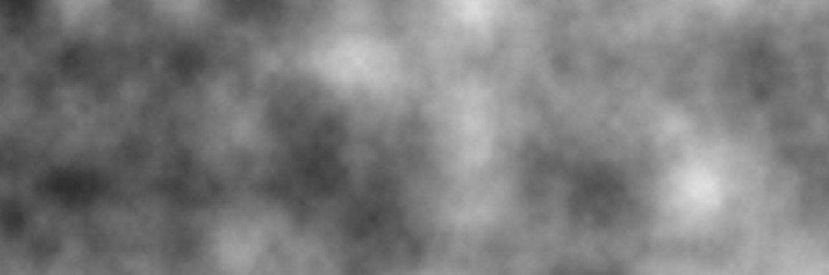
Fractal Brownian Motion (fBM)

The 2D noise snippet looks pretty good and will do for a good noise texture in most scenarios. However, if you are using the noise to portray real-world irregularities, it is too uniform and looks more like a blurred grid pattern. Real-world randomness is more dynamic. We can achieve this by adding several noise patterns together but at different sizes. This is what is commonly referred to as Fractal Brownian Motion.

By controlling how many noises we add (octaves), how intense (amplitude) and how “tight” (frequency) each layer is we get a much more dynamic noise pattern.

float random(vec2 uv) {
    return fract(sin(dot(uv.xy,
        vec2(12.9898,78.233))) *
            43758.5453123);
}

float noise(vec2 uv) {
    vec2 uv_index = floor(uv);
    vec2 uv_fract = fract(uv);

    // Four corners in 2D of a tile
    float a = random(uv_index);
    float b = random(uv_index + vec2(1.0, 0.0));
    float c = random(uv_index + vec2(0.0, 1.0));
    float d = random(uv_index + vec2(1.0, 1.0));

    vec2 blur = smoothstep(0.0, 1.0, uv_fract);

    return mix(a, b, blur.x) +
            (c - a) * blur.y * (1.0 - blur.x) +
            (d - b) * blur.x * blur.y;
}

float fbm(vec2 uv) {
    int octaves = 6;
    float amplitude = 0.5;
    float frequency = 3.0;
	float value = 0.0;
	
    for(int i = 0; i < octaves; i++) {
        value += amplitude * noise(frequency * uv);
        amplitude *= 0.5;
        frequency *= 2.0;
    }
    return value;
}

This example uses a simple 2D noise as the pattern. You can also use, for example, the Perlin noise from this snippet.